Differential equations with Python

SciPyLA 2016 - Florianópolis, Santa Catarina, Brasil - 20 de Mayo de 2016

What is a differential equation?

A Differential equation is an equation involving a depending variable and its derivatives with respect to one or more independing variables. Many laws of nature, in Physics, Chemistry, Biology, and Astronomy; are expressed in the language of Differential equations. These equations have applications not only in the physical sciences but also in applied sciences such as Engineering, Finance and Economy.

Why they are important?

It is easy to understand the reason behind this broad utility of Differential equations. if $y = f(x)$ is a given function, then its derivative $dy / dx$ can be interpreted as the rate of change of $y$ with respect to $x$. In any natural process, the variables involved and their rates of change are connected with one another by means of the basic scientific principles that govern the process. When this connection is expressed in mathematical symbols, the result is often a Differential equation.

Newton's law of cooling

The Newton's law of cooling states that the rate of heat loss of a body is proportional to the difference in temperatures between the body and its surroundings.

The law says that the rate of change in the temperature $\frac{dT}{dt}$ is proportional to the difference between the temperature of the object $T(t)$ and the temperature of the environment $T_{e}$. This can be expressed with a Differential equation, in the following way:

$$\frac{dT}{dt} = -k(T - T_{e})$$

Where $k$ is a proportional constant, $t$ is the variable time, $T_{e}$ is the environment and $T$ is our unknown function of temperature.

Differential equations classification

The Differential equations can be classified into two main groups:

• Ordinary Differential Equations

• Partial Differential Equations

Ordinary Differential Equations

The Differential equation of the Newton's law of cooling, is an example of an Ordinary Differential Equation, because of its derivatives depends of a single independent variable (time).

When a Differential equation contains derivatives with respect to a single independent variable, we call them Ordinary Differential Equations or ODE for short.

Some examples are:

$$\frac{d^2y}{dx^2} + \frac{dy}{dx} + y = 0; \hspace{2cm} \frac{dy}{dx} = 2xy; $$

Partial Differential Equations

A Partial Differential Equation is an equation that contains partial derivatives.

In the Partial Differential Equations, or PDE for short, the unknown function depends of two or more independent variables $x, y, \dots$. In general the unknown function is expressed as $u(x, y, \dots)$ and its partial derivatives as $\partial u / \partial x = u_x$ or $\partial u / \partial y = u_y$.

Some examples of these equations are:

$$\frac{\partial^2 w}{\partial x^2} + \frac{\partial^2 w}{\partial y^2} + \frac{\partial^2 w}{\partial z^2} = 0 \hspace{2cm} a^2\left(\frac{\partial^2 w}{\partial x^2} + \frac{\partial^2 w}{\partial y^2} + \frac{\partial^2 w}{\partial z^2}\right) = \frac{\partial w}{\partial t}$$

Initial and Boundary conditions

The Differential equations might have a family of solutions, but in general, we will be interested in finding a particular solution; in order to do that, we need to impose auxiliary conditions. These conditions are motivated by the physics of the problem and they come in two varieties: initials conditions and boundary conditions.

Initial condition

The initial condition specifies the physical state at a particular time, $t_0$. For example, for the diffusion problem, the initial condition will be:

$$u(x, t_0) = \phi(x)$$

where $\phi(x)= \phi(x, y, z)$ is a given function for the initial concentration. For the heat flow problem, $\phi(x)$ will be the initial temperature.

Boundary conditions

The boundary conditions will define the domain in which our PDE is valid. For example, in the diffusion problem, the domain could be define by the surface of the object holding the liquid.

There are different types of boundary conditions, the 3 more important are:

• The Dirichlet boundary condition, where the valid values for the unknown function $u$ are specified.

• The Neumann boundary condition, where the valid values are given for some of the derivatives of the function $u$.

• The Robin boundary condition, where the specified values are a linear combination of the function $u$ ard its derivatives.

Power series

When we start working on Differential equations, there are lots of cases that cannot be solved by analytic methods; but maybe we can find aproximated solutions in the form of power series.

What is a power serie?

A Power serie is a sum of terms with a infinity expansion, in general the series adopts the following form:

$$\sum_{n=0}^{\infty} C_nX^n = C_0 + C_1X + C_2X^2 + C_3X^3 + \dots $$

where $X$ is a variable and the $C_n$ are constants or the serie's coefficients. A power serie can converge for some values of $X$ and diverge for other values of $X$. The sum of the serie is a function.

$$f(x) = C_0 + C_1X + C_2X^2 + C_3X^3 + \dots + C_nX^n + \dots$$

The domain of this function is given by the values of $X$ that make the serie converge.

Taylor Serie

The Taylor series are special cases of power series with the terms expressed by the form $(x - a)^n$. The Taylor series allow us to aproximate continous functions that cannot be solved by the analytic method. Taylor series are constructed by the derivatives of these functions. Its mathematical definition is:

$$f(x) = \sum_{n=0}^{\infty}\frac{f^{(n)}(a)}{n!}(x - a)^n$$

which is equivalent to:

$$f(x) = f(a) + \frac{f'(a)}{1!}(x -a) + \frac{f''(a)}{2!}(x -a)^2 + \frac{f'''(a)}{3!}(x -a)^3 + \dots$$

The Taylor series are important because they allow us to integrate functions that we cannot handle in other way.

Analytic solutions with Python

SymPy

SymPy

SymPy is a Python library for symbolic mathematics. It aims to become a full-featured computer algebra system (CAS).

Some of its features are:

• Basic algebra: Simplifications, expansions, sustitutions, arithmetic...
• Calculus: Limits, derivatives, integrals, taylor series...
• Equation solvers: Algebraic equations, polynomial equations, differential equations, systems of equations...
• Matrices: Determinants, basic arithmetic, eigenvalues, eigenvectors...
• Physics: mechanics, quantum mechanics, optics, Pauli algebra
• Other.

Problem to solve

Suppose there was a murder and police arrives to the crime scene at 2:41 am. The forense takes the temperature of the victim and found to be 34.5 ° C; then take the temperature again an hour later and the reading mark 33.9 ° C.

Assuming that day the weather was warm and the evironment had a constant temperature of 15 ° C.

What was the time of the murder?

Solving the problem by the analytic method with SymPy

In order to solve this problem we can use the Newton's law of cooling differential equation.

Our data are:

• Initial temperature = 34.5
• Temperature after 1 hour = 33.9
• Environment temperature = 15
• Average temperature of a human being = 37

# unknows definitions
t, k = sympy.symbols('t k')
y = sympy.Function('y')

# express equation.
f = k*(y(t) -15)
sympy.Eq(y(t).diff(t), f)

$$\frac{d}{d t} y{\left (t \right )} = k \left(y{\left (t \right )} - 15\right)$$

# Solving the equation
edo_sol = sympy.dsolve(y(t).diff(t) - f)
edo_sol

$$y{\left (t \right )} = C_{1} e^{k t} + 15$$

Now, we have the solution of the differential equation, in order to find out the integration constant we need to use the initial condition.

# Initial condition.
ics = {y(0): 34.5}

C_eq = sympy.Eq(edo_sol.lhs.subs(t, 0).subs(ics), edo_sol.rhs.subs(t, 0))
C_eq

$$34.5 = C_{1} + 15$$

C = sympy.solve(C_eq)[0]
C

$$19.5$$

Now, we have the value of C, the next step is to find out the value of $k$.

eq = sympy.Eq(y(t), C * sympy.E**(k*t) +15)
eq

$$y{\left (t \right )} = 19.5 e^{k t} + 15$$

ics = {y(1): 33.9}
k_eq = sympy.Eq(eq.lhs.subs(t, 1).subs(ics), eq.rhs.subs(t, 1))
kn = round(sympy.solve(k_eq)[0], 4)
kn

$$-0.0313$$

We have all the data, so we can try to find out the approximation of the murder's time.

hmuerte = sympy.Eq(37, 19.5 * sympy.E**(kn*t) + 15)
hmuerte

$$37 = 19.5 e^{- 0.0313 t} + 15$$

t = round(sympy.solve(hmuerte)[0],2)
t

$$-3.85$$

h, m = divmod(t*-60, 60)
print "%d horas, %d minutos" % (h, m)

3 horas, 51 minutos

That is, they spent about 3 hours and 51 minutes after the crime have occurred, therefore the time of the murder was around 10:50 pm.

Power series and direction fields

Now, suppose that we want to solve with SymPy the following differential equation:

$$\frac{dy}{dx} = x^2 + y^2 -1$$

with the initial condition of $y(0) = 0$.

Using the same method as before, we get the following result:

# unknown definitions
x = sympy.symbols('x')
y = sympy.Function('y')

# function definition
f = y(x)**2 + x**2 -1

# Condición inicial
ics = {y(0): 0}

# solving ode
edo_sol = sympy.dsolve(y(x).diff(x) - f, ics=ics)
edo_sol

$$y{\left (x \right )} = - x + \frac{2 x^{3}}{3} - \frac{4 x^{5}}{15} + \mathcal{O}\left(x^{6}\right)$$

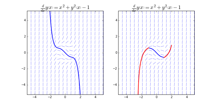
The result that SymPy gives us, is an approximation with power series (Taylor serie); and the problem with the power series is that their results are often only valid for a certain range of values. One tool that can help us visualize the range of validity of an approximation with power series are the Direction fields.

Direction fields

The Direction fields is a simple but useful technique to visualize possible solutions to arbitrary first-order ODEs. It is made up of short lines that show the slope of the unknown function on a grid in the $x–y$ plane. This graph can be easily produced because the slope of $y(x)$ at arbitrary points of the $x–y$ plane is given by the definition of the ODE:

$$\frac{dy}{dx} = f(x, y(x))$$

That is, we only need to iterate over the $x$ and $y$ values on the coordinate grid of interest and evaluate $f(x, y(x))$ to known the slope of $y(x)$ at that point. The direction lines in the Direction fields suggest how the curves that are solutions to the corresponding ODE behave, and direction field graphs are therefore a useful and tool for visualizing solutions to ODEs that cannot be solved analytically.

For example, the direction field of for the equation:

$$\frac{dy}{dx} = x^2 + y^2 -1$$

is the following:

# Direction field plot
fig, axes = plt.subplots(1, 1, figsize=(7, 5))
campo_dir = plot_direction_field(x, y(x), f, ax=axes)

Range of validity of the solution with power series

Now that you know the Direction fields graph, we can go back to the approximate solution with Power series that we had obtained previously. We can plot the solution in the Direction fields , and compared it with a numerical solution method.

In the left panel, we see that the approximate solution curve aligns well with the direction field lines between -1.5 and 1.5 values of $x$, but then it starts to deviate, suggesting that the approximate solution is no longer valid. The solution curve shown in the right panel aligns better with the direction field throughout the plotted range.

Numeric solutions with Python

SciPy

SciPy

SciPy is one of the core packages that make up the SciPy stack. It provides many user-friendly and efficient numerical routines such as routines for numerical integration and optimization. Some of the modules included in the package, are:

• scipy.integrate: That provides different functions for solving numerical integration.
• scipy.linalg: That provides functions for solving linear algebra.
• scipy.optimize: for optimization and minimization problems.
• scipy.signal: for signal processing and analysis.
• scipy.sparse: for sparse matrices and solving sparse linear systems.
• scipy.stats: for statistics and probability analysis.

To solve Differential equations, we will us the module scipy.integrate.

Solving Differential equations with SciPy

SciPy offers two ordinary differential equations solvers, integrate.odeint and integrate.ode. The main difference between them is that integrate.ode is more flexible, offering us the choice between different solvers; but integrate.odeint is easier to use.

We will try to solve the following equation:

$$\frac{dy}{dx} = x + y^2$$

# function defintion
f = y(x)**2 + x
f

$$x + y^{2}{\left (x \right )}$$

# lambdify sympy function.
f_np = sympy.lambdify((y(x), x), f)

# initial conditions and x range. 
y0 = 0
xp = np.linspace(0, 1.9, 100)

# calculating numeric solution to y0 and xp
yp = integrate.odeint(f_np, y0, xp)

# same calculation for negative values.
xn = np.linspace(0, -5, 100)
yn = integrate.odeint(f_np, y0, xn)

The results are two one-dimensional NumPy arrays $yp$ and $yn$, of the same length as the corresponding coordinate arrays $xp$ and $xn$, which contain the numerical solution to the ODE problem at the specified points. To visualize the solution, we next plot the $yp$ and $yn$ arrays together with the direction field for the ODE.

# ploting solution with direction field.
fig, axes = plt.subplots(1, 1, figsize=(8, 6))
plot_direction_field(x, y(x), f, ax=axes)
axes.plot(xn, yn, 'b', lw=2)
axes.plot(xp, yp, 'r', lw=2)
plt.show()

System of Differential equations

In previous example, we solved only one equation. Generally, most problems arise in the form systems of ordinary differential equations, that is, it include several equations to be solved. To see how we can use integrate.odeint to solve such problems, consider the following system of ordinary differential equations, known Lorenz equations:

$$x'(t) = \sigma(y -x), \\ y'(t) = x(\rho -z)-y, \\ z'(t) = xy - \beta z $$

These equations are known for their chaotic solutions, which sensitively depend on the values of the parameters $\sigma$, $\rho$ and $\beta$. Let see how can be solved using Python.

# System of equation definition
def f(xyz, t, sigma, rho, beta):
    x, y, z = xyz
    return [sigma * (y - x),
           x * (rho - z) - y,
           x * y - beta * z]

# parameters values
sigma, rho, beta = 8, 28, 8/3.0

# initial condition and range of solutions.
xyz0 = [1.0, 1.0, 1.0]
t = np.linspace(0, 25, 10000)

# Solving the equations
xyz1 = integrate.odeint(f, xyz0, t, args=(sigma, rho, beta))
xyz2 = integrate.odeint(f, xyz0, t, args=(sigma, rho, 0.6*beta))
xyz3 = integrate.odeint(f, xyz0, t, args=(2*sigma, rho, 0.6*beta))

# plotting the solutions
from mpl_toolkits.mplot3d.axes3d import Axes3D
fig, (ax1,ax2,ax3) = plt.subplots(1, 3, figsize=(12, 4),
                                  subplot_kw={'projection':'3d'})

for ax, xyz, c in [(ax1, xyz1, 'r'), (ax2, xyz2, 'b'), (ax3, xyz3, 'g')]:
    ax.plot(xyz[:,0], xyz[:,1], xyz[:,2], c, alpha=0.5)
    ax.set_xlabel('$x$', fontsize=16)
    ax.set_ylabel('$y$', fontsize=16)
    ax.set_zlabel('$z$', fontsize=16)
    ax.set_xticks([-15, 0, 15])
    ax.set_yticks([-20, 0, 20])
    ax.set_zticks([0, 20, 40])

Partial Differential Equations

Until now, we only see Ordenary Differential Equations, but What about Partial Differential Equations?

This kind of equations are much more hard to solve; one powerful method we can use is the Finite Elements Method and try to find out a numerical solution.

Finite Elements Methods

The basic idea of FEM is to divide the body into finite elements, often just called elements, connected by nodes, and obtain an approximate solution of the partial differential equation. This new object is called the finite element mesh.

To ilustrate, lets see an example, suppose that we have a plate with a hole and we want to calculate its heat distribution. To accomplish that, we need to solve the heat equation for each point in the plate. The approach that the Finite Elements Methods use, is to divide the object in finite elements interconected by the nodes. This new object is the mesh and it is and approximation of the original object. The more nodes we have, the more accuate the solution will be.

The FEniCS project

the FEniCS is a highly capable FEM framework that is made up of a collection of libraries and tools for solving PDE problems. Much of FEniCS is programmed in C++, but it also provides an official Python interface.

We can install it in Ubuntu with the following command:

sudo add-apt-repository ppa:fenics-packages/fenics
sudo apt-get update
sudo apt-get install fenics

The main interface for working with the framework are the libraries dolfin and mshr; so we will need to import both modules. Take into acount that FEniCS only works with Python 2.

The problem

The problem we will solve with FEniCS help, is the steady-state heat equation defined by:

$$u_{xx} + u_{yy} = f$$

where $f$ is the source function and with the following boundary conditions:

$$u(x=0) = 3 ; \ u(x=1)=-1 ; \ u(y=0) = -5 ; \ u(y=1) = 5$$

The first step in the solution of a PDE with FEM is to define a mesh that describes the discretization of the problem domain. In the current example the problem domain is the unit square $x, y \in [0 , 1]$. For simple geometries like this, we use the RectangleMesh function from the dolfin module.

# discretization of the problem.
N1 = N2 = 75
mesh = dolfin.RectangleMesh(dolfin.Point(0, 0), dolfin.Point(1, 1), N1, N2)

# mesh plot
dolfin.RectangleMesh(dolfin.Point(0, 0), dolfin.Point(1, 1), 10, 10)

The next step is to define a representation of the function space for the trial and the test functions, using the dolfin.FunctionSpace class. The constructor of this class takes at least three arguments: a mesh object, the name of the type of basis function, and the degree of basis function. For our purposes we will use the Lagrange type of basis functions of degree 1.

# base functions
V = dolfin.FunctionSpace(mesh, 'Lagrange', 1)
u = dolfin.TrialFunction(V)
v = dolfin.TestFunction(V)

DEBUG:FFC:Reusing form from cache.

Now, we can transform our PDE to the weak form and reduce it to a linear algebra problem we can solve using the FEM.

# PDE weak formulation
a = dolfin.inner(dolfin.nabla_grad(u), dolfin.nabla_grad(v)) * dolfin.dx
f = dolfin.Constant(0.0)
L = f * v * dolfin.dx

and we define the boundary conditions.

# boundary conditions
def u0_top_boundary(x, on_boundary):
    return on_boundary and abs(x[1]-1) < 1e-8

def u0_bottom_boundary(x, on_boundary):
    return on_boundary and abs(x[1]) < 1e-8

def u0_left_boundary(x, on_boundary):
    return on_boundary and abs(x[0]) < 1e-8

def u0_right_boundary(x, on_boundary):
    return on_boundary and abs(x[0]-1) < 1e-8

# Dirichlet boundary conditions
bc_t = dolfin.DirichletBC(V, dolfin.Constant(5), u0_top_boundary)
bc_b = dolfin.DirichletBC(V, dolfin.Constant(-5), u0_bottom_boundary)
bc_l = dolfin.DirichletBC(V, dolfin.Constant(3), u0_left_boundary)
bc_r = dolfin.DirichletBC(V, dolfin.Constant(-1), u0_right_boundary)

# list of boundary conditions
bcs = [bc_t, bc_b, bc_r, bc_l]

Now, we can solve the PDE using the function dolfin.solve. We can convert the resulting vector to a NumPy array and then plot the solution using Matplotlib.

# Solving the PDE
u_sol = dolfin.Function(V)
dolfin.solve(a == L, u_sol, bcs)

# plotting the solution
u_mat = u_sol.vector().array().reshape(N1+1, N2+1)

x = np.linspace(0, 1, N1+2)
y = np.linspace(0, 1, N1+2)
X, Y = np.meshgrid(x, y)

DEBUG:FFC:Reusing form from cache.
DEBUG:FFC:Reusing form from cache.

fig, ax = plt.subplots(1, 1, figsize=(8, 6))

c = ax.pcolor(X, Y, u_mat, vmin=-5, vmax=5, cmap=mpl.cm.get_cmap('RdBu_r'))
cb = plt.colorbar(c, ax=ax)
ax.set_xlabel(r"$x_1$", fontsize=18)
ax.set_ylabel(r"$x_2$", fontsize=18)
cb.set_label(r"$u(x_1, x_2)$", fontsize=18)
fig.tight_layout()

Other solvers

Other solvers for PDE in Python are:

• SfePy: Simple Finite Elements in Python.

• FiPy: A Finite Volume PDE Solver Using Python.

Links

• Introducción al cálculo con python
• Ecuaciones diferenciales con python
• Ecuaciones en derivadas parciales con python
• SymPy
• SciPy
• proyecto FEniCS
• SfePy
• FiPy
• Numerical Python - Robert Johansson

Thanks!

Raul E. Lopez Briega

https://relopezbriega.github.io/

Twitter: @relopezbriega

Slides: https://relopezbriega.github.io/ecuaciones-diferenciales-en.html